Understanding India’s ‘Federalism’, and 2020’s Fiscal Troubles
India enters the "Municipal Quantitative Easing" Era
This is a Guest Article for Notes on the Crises. Thanks to the generous support of our paid subscribers, we can now afford to have guest writers
Advait Moharir is a Research Assistant at Azim Premji University. He is currently working on the CORE Project, helping develop materials for an economics textbook being written for the South Asian context. His interests lie in the fields of macroeconomics, monetary economics and public finance.
Publisher Note: Some wrote in after Advait’s last guest piece, asking me to explain why I’m interested in publishing this kind of analysis. For one thing, India is a very important country with a very large population that is worth better understanding. Second, important differences between how public finance works in the United States versus in India are informative about the uniqueness of our system. Comparisons can illuminate other possible ways we could approach public finance. In particular, the higher degree of centralization of sub-national finance in India is extremely interesting, for reasons Advait contextualizes below. Finally, the similarities between India and the United States in the realm of public finance helps us think through what lessons India may be able to take from the U.S. experience. I’m especially struck by the fact that the Indian central bank just this week announced purchases of state debts, moving monetary policy in a direction that the Federal Reserve has gone in. Finally, as I discussed in this week’s premium piece on Federal Reserve swap lines, I’m interested in gradually discussing more of the neglected geopolitics of international monetary policy. This will allow us to gain a better understanding of the internal politics of important countries like India, and the world as a whole.
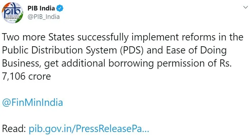
On 2nd October, the Press Information Bureau, India’s nodal government agency which announces its policy decisions, tweeted the following statement:

The tweet says a lot more than meets the eye. What can this brief statement tell us about India’s sub-national debt management?
The extent to which states in India can borrow is conditional on them implementing certain policies (or ‘reforms’). The essentially hierarchical nature of Centre-State relationships in India is revealed here — whether the policies are agreeable to the state government, or if they are suitable to those contexts is completely irrelevant. The power to borrow is intrinsically linked to the relationship of the state with the existing Central government. This has implications we will return to later in the article.
As Notes on the Crises regular readers will remember, I’ve written an article analyzing the factors that drive India’s public debt. My findings were at odds with more orthodox economists working on India — using a simple equation of debt movement, I found that more than two-thirds of the change in India’s debt/GDP ratio is explained by the difference in the interest rate and the growth rate. In other words, the changes in the debt ratio are not primarily led by new borrowing.
However, a comprehensive understanding of public debt in India requires a deep dive into sub-national debt. The FRBM Review Committee (which I mentioned in my last guest piece) stated that the total debt to GDP ratio should be pinned at 60%. 40% of this debt will be borne by the Centre, while 20% will be borne by the states. This particular division of the target raises many questions — Is the 20% a ratio of all the states’ GDP, or is it a fraction of each of their state domestic products? Is there a specific coordinating mechanism to ensure this target is met within the deadline? But the most important question outstanding is: which states will have to cut spending, and which states can continue to stimulate their economies? This becomes an important issue in the middle of the pandemic, as 60% of coronavirus cases come from only five states.
The tweet in the beginning also raises an important question — what kind of political structure allows the Centre to have such conditional checks on local government finances? To understand this, let us take a short look at India’s federal system.
Federalism in India
India follows a model of “coming together” federalism — in theory, multiple entities coming together to form a Union. However, the whole is made up of many incongruent and often contesting parts. In India’s case, the Centre is vested with much more authority over the states than we might expect from a federal model of governance. This is why India is sometimes called a ‘quasi’-federal entity. An embodiment of this power is the Finance Commission — this is a body which determines the distribution of tax generated revenue between the Centre and the States. It also sets the basis for how grant aid is to be granted to states, among other things. This is very different from the system in, say the US, where each State has power to levy its own taxes. So perhaps understanding India as ‘federal’ is misleading, or at least not the whole story.
This lop-sided concentration of power often leads to conflicts. A recent manifestation of this is the on-going conflict between the two on the covering of shortfall in tax revenue. By establishing a unified Goods and Services Tax, several indirect taxes have been eliminated, leading to revenue loss for the states. This shortfall was to be covered by a consolidated fund. However, the Centre is attributing part of the revenue loss over the last year as partly due to COVID-19 (calling it “act of god”). As such, they’re demanding that the states borrow the full or partial amount directly from the market, to make up for the shortfall. As expected, a lot of states are demanding that by yielding their powers to levy taxes, and the onus is on the Central government to borrow. While some states have agreed to borrow, others remain defiant, and the issue remains unresolved.
Another example is the conditional borrowing referred to in the tweet. The power to establish the terms for borrowing is vested by Article 293(3) of the Constitution, which states:
“A State may not without the consent of the Government of India raise any loan if there is still outstanding any part of a loan which has been made to the State by the Government of India or by its predecessor Government, or in respect of which a guarantee has been given by the Government of India or by its predecessor Government”
In simple words, there is no way for States to borrow in unfettered ways. Moreover, Article 293(4) allows the Central government to impose whatever conditions it sees fit.
It is no coincidence that the two conditions, namely the linking of the public distribution system to a unique identity card, and reshaping the local economy to align with the ease of doing business index, are major policy planks of the current regime. The presence of regional political parties — which often have opposing political ideologies — further complicates this matter. Both these policies are seen as an infringement of autonomy of state governments, as well as an attempt to force a particular kind of economic ideology on the states.
It is interesting to note that both examples leave the States with limited options. The Centre is asking the states to borrow to cover up the revenue shortfall on one hand. At the same time, it is also placing significant constraints on borrowing from the Centre. The onus of borrowing is shifted onto the states, whilst a key source of funding — the Centre itself — is effectively cut off. The unequal power dynamics arising out of this brand of federalism are essential to understanding subnational debt.
With this background, let us now tackle the question of how subnational debt has evolved over time. Again, the framework I use to assess this question is outlined in my previous article for Notes on the Crises.
Subnational debt dynamics
Similar to the last article, I decomposed the change in debt due to two factors — new borrowing, and the interest-growth differential (i-g). Table 1 shows the results of this decomposition for the collective debt ratio of the ten biggest states by population. Since these account for 75% of all liabilities, they are fairly representative:

For the most part (1992- 2013), i-g drives subnational debt. However, from 1981-91, and at present, new borrowing is driving the change. This is what makes the subnational case from the national case, where i-g drove debt change in all periods. The reason for this difference is simple — the i-g dynamics were strong enough in the previous period (2005-13), that the debt ratio fell. Indeed so much that these figures show that where the magnitude of primary deficit was larger than the magnitude of i-g on previous debt. This was decisive. It is important to note that g>r throughout, meaning that the debt ratio will not rise indefinitely.
While the overall decomposition does give some limited credibility to the calls for austerity, it raises a thorny question — which states will be the one to cut spending, and by how much? Considering this question that all but extinguishes the orthodox account of India’s debt. The argument that the states together need to reduce their debt ratio to 20% would only make sense if the states were a country of their own! The Report is conspicuously silent on this matter — it does not specify the distributional consequences of a uniform fiscal rule.
In simple words, how does one apply a single rule to different states, with different socio-economic backgrounds?
To answer this question, I did the debt decomposition of each of these ten states, with the debt measured as a ratio of state domestic product. In six out of the ten states, i-g was the dominant cause of debt change overall. Meanwhile, in five out of the ten states, primary deficits became the dominant explainer in the last period. Clearly, some states can continue spending, while some will have to pull up their purse strings to meet their 20% target. How does this pan out in the future?
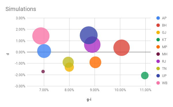
Chart 1 shows the simulated value of the constant level of new borrowing/lending each state will have to undertake to go from their current debt ratio to 20% over the next five years. This is plotted against their average (i-g). The size of the bubbles is relative to the size of their debt ratio. A very clear pattern emerges — states with smaller debt ratios can continue to borrow more (indicated by negative d), while states with larger debt ratios will have to cut spending. This is not all. The states which can spend more are also the more prosperous states, with stronger institutions. By contrast, the states which will have to undertake austerity, are the ones which are less prosperous, not well governed, and fare badly in terms of most socio-economic indicators.
Of course, we know from international experience with International Monetary Fund structural adjustment programs, what is considered “poor governance” covaries with other socioeconomic indicators and doesn’t cause low incomes or budget deficits. Meanwhile, the consequences of imposing a homogenous fiscal rule are damaging—poor states will withdraw spending and spiral towards lower output. At the same time, the richer states can continue spending and remain prosperous. To put the most likely outcome in simple terms: regional inequality will worsen. Poverty in weaker States will entrench.
This also has short-term consequences to the pandemic response. A state like Maharashtra with favourable dynamics can continue spending unfettered. But a state like Andhra Pradesh will have to maintain a balanced budget, and cut expenditure. A state like Uttar Pradesh, however will suffer the most — it has to maintain a primary surplus (become a net lender!) of almost 1.5%. But it also has to deal with 47,000 plus active cases. As has historically been the case, these disparities will tend to widen and amplify over time.
Can Monetary Policy be used to manage debt?
Over the last two articles, I have explored the determinants of the evolution of national and subnational debt in India. At this juncture, it is important to note the following —
- First, over the last thirty years or so, the debt ratio has been driven by factors other than new borrowing-mainly the interest rate- growth differential.
- Secondly, fiscal rules have played a key rule in curtailing expenditure at both levels, while the federal structure has amplified these difficulties at the subnational level.
- Finally, monetary policy seems to be the preferred route taken by policymakers, with the RBI taking a relatively proactive role.
The final point needs some elaboration. As mentioned in the previous article, the RBI has cut the repo rate by 115 basis points (or 1.15%) over the last four months-making them the steepest and fastest rate cuts over the last few decades. However, have changes in the repo historically spilled-over to change the interest rate on government borrowing?

Chart 2 shows the movement of the repo rate against the movement of the weighted average of interest rates on bonds issued by the Centre and the States. While they are not correlated perfectly, all three rates move closely together, with some divergence in the early 2000s, and after the 2008 crisis. The difference in bond rates and repo rate can be interpreted as a “risk premium”- the repo is a risk-free asset, and typically, the higher interest payments on other assets (the G-secs in this case), are a measure of the perceived additional risk. This is why, overall, the repo rate is lower than the bond yields. However, in July, August and September 2020 (not part of Chart-2), the repo rate is at 4%, while the yield of the 364-day bond is lower at 3.5%. This negative risk premium, is probably largely due to the fall in oil prices, which form a significant component of the premium, according to a RBI Working Paper. Overall, the RBI has significant control over bond yields, and this strong relationship strengthens the case for using monetary policy as a tool for debt management.
A recent development merits a mention here- On 9th October, the RBI Governor announced that the Bank will purchase bonds issued by the State government. This is the first time such a move has been announced, and in the words of the governor was done to ensure a “smooth and seamless transmission of monetary policy impulses as well as the completion of market borrowing programmes of the centre and states…”. By reducing the repo rate over time, and the announced purchase of state debt, the central bank has reduced the cost of borrowing. Although this is not sufficient by itself, it will reduce (i-g), bringing much-needed relief to the states. However, the distributional questions remain- which states will be preferred, and what will be the quantum of borrowing from each? These questions assume more significance in light of the discussion on regional inequality in the previous section. The RBI must soon bring out a short discussion paper explaining how it plans to proceed, especially given that this is the first time it is carrying out such an exercise.
Conclusion
The dual combination of a quasi federal structure and fiscal rules have encumbered the state’s ability to borrow. While it is impractical to think about changing the federal structure itself, the Centre does have the option of using the framework to ease borrowing mechanisms. Until the pandemic eases at least, all conditionalities on state borrowings from the centre must be removed.
This measure would up the states to a key source of funding, and remove the pressure of pursuing structural change in the short-term. As far as the GST compensation issue is concerned, there is no one answer. If the insistence on fiscal prudence remains, then some states can borrow directly, while the Centre will have to borrow for states with high debt and low growth. Parallelly, the GST legislation itself needs re-working, so that its relationship to Article 293 (the law that gives the Centre allocatory power) is defined clearly, and the States have easier means of borrowing, especially during crises.
This brings us to the bigger question of the role of fiscal rules itself. The 3% rule was ineffective in regulating spending. With the coronavirus pandemic throwing all well-laid plans into disarray, it does not seem likely that the 60% target is viable anytime in the near future. More importantly, these targets are completely arbitrary — both have been borrowed from the European Union debt sustainability framework, and the government has given no reasoning for the establishment of these rules — other than the fact that they are easy to communicate to the public. The achievement of an arbitrary target of “sustainability” is secondary to the more urgent and real issues of ending the pandemic, reducing unemployment, and restarting the economy. India is fighting a phantom problem in the midst of a crisis, and it needs to stop.
Sign up for Notes on the Crises
Currently: Comprehensive coverage of the Trump-Musk Payments Crisis of 2025